

Acoustic Localization.
- Michael Maggs

- May 23, 2022
- 12 min read
Updated: Nov 28, 2024
Thinking about doing an acoustic localization project? We’d love to hear from you! Contact Michael and let’s have a chat.
This page includes the following topics:
Introduction
Acoustic localization is the practice of using the time difference of arrival (TDoA) of sounds heard by multiple recorders to work out the location of the sound source. In the world of bioacoustics, that means locating in 3D space exactly where the animal was when it called.

We really believe in the potential of acoustic localization and we’re putting in a lot of development effort into this area because we’re excited to see the science that come out of it. From changing point count surveys into actual counts of individuals, behavioural studies, or calculating the sound pressure level (SPL) of any animal call, to name just a few of the potential activities.
So grab some BAR-LT recorders and let’s get started.
Need to know
Accurate localization is all about accurate timing. If used correctly, you should reliably get <1ms timing accuracy on all recordings at any point in time for the entire length of your deployment, which may be weeks, months or more depending on your recording schedule.
Adhere to the following points and you should expect good results. And as always, if you have any questions or problems, please contact our chief engineer Michael at michaelm@frontierlabs.com.au.
Firmware: For the moment, you need to be running special firmware that enables the millisecond accurate GPS time synchronisation. In future this will be part of the normal release firmware that everyone has, but for now please email Michael to get a copy of the localization firmware.
GPS: The recorders need to be able to get GPS signals where they are being used. So caves or deep ravines will probably not work, and you may have to allow for more time to get a fix under a dense forest canopy.
Recording schedule: Keep the recording lengths >= 5 minutes and <= 1 hour. This gives the recorders enough time to synchronise but not too long for their clocks to drift more than 1ms. If you want to record continuously, just make the schedule event repeat with the same repeat period as the recording duration, i.e. record for 1 hour every hour.
Settings: The sample rate and channel of the recording must be 44.1kHz, mono. This will change in future but for now make sure you use these settings.
Deployment: You should have some means to measure to positions of the recorders using an external differential GPS, or even just the relative positions are fine, using a tape measure or a laser range finder. The onboard GPSs are not good enough to give 1m accuracy that you will need for this purpose.
Temperature: Allow your recorders to reach ambient temperature first (or have <1hr recording times). Crystal drift is temperature dependant, and recent experiments showed 1-10ms error over the first 2 hours as the recorders warmed up from an air-conditioned office to outside in full sun. After their temperatures had settled the synchronisation accuracy stayed below <1ms.
Data processing: The clock crystal drift must be compensated for during the data processing stage by stretching or compressing the length of the data to match the beginning and end timestamps in the file name. I have some software that does this if you would like to use it. See Processing your Data.
Extra Power Consumption
GPS consumes a lot of power to run, almost doubling the power consumption of the recorder, so we only turn the GPS on at the start of each recording long enough for it measure its offset and drift relative to the caesium atomic clocks in the GPS satellites. This typically takes less than a minute, however there is no maximum bounded time. If the schedule is set for 1 hour long recordings and it takes 1 minute of double power consumption to synchronise then the overall power consumption would be multiplied by a factor of:
1+1/60 = 1.0166667
This is only an increase of 1.67%, which is actually a pretty great because it means you can run a localization project without it dramatically reducing your deployment time!
Choosing your Array Geometry
There is no single best size or arrangement of recorders for all applications however you should consider the following points when planning your array:
The sound you want to locate must be recorded by at least 3 recorders for triangulation to work. Therefore, recorders cannot be further apart than the detection range of the target animal. The sensitivity of the BAR-LT recorders is close to that of a human, so if you have firsthand field experience or anecdotal evidence of how far away you can hear a call from then this may be fine if you know it is larger than your planned array size. Keep in mind that wind and pose direction of the animal can have a significant effect on the detection range. Check out How far can my recorder hear? for more information.

The closer the recorders are to each other, the smaller the differences in arrival time will be. Which means the relative size of the clock synchronisation errors compared to the size of the distance measurements will be higher.
Target sounds can be inside or outside of the border of the array.
The geometry of the array does not have to be a precise or perfect shape, like a square for example, however it is good to try to have them regularly spaced so that there is at least some evenness or symmetry to any errors in the localization calculations. Rectangles, squares, 2D grids and 3D grids are all good options.
In reality, the challenges of your field site like terrain, rocks and trees etc will all affect where you can put your recorders, so don’t worry if the geometry is not perfect as long as you can measure it.
In fact, no matter what you decide for your array geometry, it is important that you know the locations of each recorder with as much accuracy as possible.
Measuring your Array Geometry
It is important to know the position of the recorders in your array, or at least their relative geometry since they are the anchor points for the triangulation calculations. However, this is often the most practically challenging stage due to difficulties in terrain, limited line of sight to the recorders, and limitations of equipment. Many GPS systems only guarantee +/- 10m of accuracy and this is made more difficult by terrain, tree cover and weather. For most applications the on-board GPS in the BAR-LT recorders is not accurate enough. If possible, consider the following methods for measuring your array geometry:
DGPS: If you have access to a Differential GPS and can get a good signal in your target area, then this is the ideal scenario.
Laser rangefinder / tape measure: Using a laser rangefinder or other tape measure like device will give you the relative distances between each recorder which you can then use to triangulate their positions.
Acoustically: This method is less ideal than a directly measuring the distances between recorders as it will also include any time synchronisation errors in the system (which is typically <1ms or around 35cm). However, if you are unable to measure your array by the other means this will do. Follow the steps in the next section called Ground Truthing to work out the distances between each recorder.
Ground Truthing
Ground truthing your setup is an excellent way to know you've done everything right. It also allows you to directly measure the accuracy of the whole system and your triangulation calculations.
You should always perform these steps at the beginning of any localization experiment so you can have confidence in the rest of your results.
Setup you array of recorders, and make sure they are all recording.
Get as close as possible to one of the recorders and make a loud sound like a clap that can be heard by the other recorders.
Move to each of the recorders in your array and repeat this step.
In post processing, the direct path of the sound to the other recorders can be measured by the difference in arrival times of the sound and converted directly into a distance measurement without having to do any triangulation maths. You can then compare this directly with the measured distances between each recorder.

It is also a good idea once the array is up and recording to log a few other GPS points in your study area and make loud sounds there. That way you can measure the accuracy of the whole triangulation process as well by comparing the computed positions to the measured positions.
Processing your Data
There are many different options and approaches for processing acoustic localization data. However, there is one important point to keep in mind when processing data from our recorders:
The duration of the data must be stretched to fit the start and end times listed in the filename (and meta data).
i.e. The sample rate clock is not adjusted to match the atomic GPS clocks. Instead, we measure the clock drift error and compensate it in post processing.
Why do we do it this way? (click the arrow to find out)
Crystal oscillators (the beating heart of nearly all modern clocks) are not perfect and have some small amount of error measured in parts per million (PPM). For example, a crystal with a tolerance of 10PPM can lose up to 10s every Million seconds, or roughly 1s every day. This doesn’t sound like much but if you’re trying to achieve ms level synchronisation this adds up fast. In fact, over a 1 hr recording this amounts to 36ms! Trying to adjust and compensate for this drift in hardware causes jitter in the time readings, so instead we simply measure the drift as accurately as possible and compensate for it in post processing, which gives much more accurate and stable results.
We have software that does this automatically, however if you are already using a different software package and need to do this manually, the start and end times of each file is encoded into the filename in ISO8601 format and stored in the meta-data using the GUANO format.
Below is an example filename with the start and end times and GPS position highlighted.
S20220408T155959.129679+1000_E20220408T165954.067716+1000_-27.54336+153.02912.wav
Start time: 2022/04/08 15:59:59.129679 local time in time zone UTC+10:00
End time: 2022/04/08 16:59:54.067716 local time in time zone UTC+10:00
GPS location: -27.54346+153.02862
By saving the start and end times of the recordings, clock drift errors can be accounted for by stretching or compressing the time axis of the data to match the real duration of the recordings according to GPS time. If you are working with a process that requires multi-channel wav files, then the samples will need to be interpolated to match the “real” sample rate.
The software we have developed does not require the files to be interpolated as it automatically stretches or compresses the data independently for each recording. It also allows you to select a file from one recorder and it will then display the corresponding file from all the other recorders in the array, and then display them all aligned in the “real-time” axis, regardless of the start times of the files.
The figure below shows recordings from an array of 4 recorders. Selecting a different file from one recorder automatically updates the view of the other recorders to show the audio happening at that time from those recorders. In this test all the microphones were placed in the same spot, so the sounds arrived at the same time. Here the recoded synchronisation accuracy was measured as 0.03ms, or 30us

Drift compensation happens automatically by stretching the time axis of each recording based on the real start and end times logged in the filename and meta-data of each file. If drift compensation is disabled, or you are using another piece of software to look at the data then you will notice a large synchronisation error accumulate by the end of a 1 hour recording. The figure below shows the same recordings as Fig 4, except with drift compensation disabled, resulting in an accumulated synchronisation error of 41.29ms after 1 hour.

Using the Acoustic Localization software
Firstly, you should copy all your SD cards onto a drive and put them into a sperate folder for each recorder. It is important to copy over everything from the SD cards, include all log files and loclog.txt files. If there are multiple SD cards per recorder, put them into a single folder for that recorder. The software will scan through each folder and subfolder and find all the associated wav files and log files.
Using our Acoustic localization software, a typical workflow for a project consists of the following 3 steps:
1. Add the recorders to your project.
2. Refine the recorder positions.
3. Localize sounds.
These are described in detail below.
Add recorders to the array:
Click the Add a Recorder button from the main menu or click on the [ + ] button in the Recorders table.

Select the base directory that contains all the data from a recorder. Click OK and the recorder will appear on the Map View and the audio will start to load in the Audio View.
Repeat this for all recorders in your array.

Refine the recorder positions:
If you performed the position calibration (step 2) during the deployment, then you can convert the time-difference-of-arrival of those sounds into physical distance constraints between the recorders:
In the Audio View tab, find one of the calibration sounds you made during the deployment (you can zoom in on the spectrogram to get a better view) and draw a box around it. The selected audio (show in green) will be filtered according to the bounding box you draw on the spectrogram. You can press the play button to verify it is the correct sound. Purple search boxes will automatically appear in the recordings from other units, these can be manually adjusted or removed by right clicking anywhere in that audio view.

Click the Match Audio Selection button from the main menu or click on button in the Distance Constraints table header in the Side Panel.

This will search for the snippet of audio in the purple search windows from the other recorders. The results will be shown in yellow along with the relative time differences relative to "real time" not "file time". You can zoom in and adjust the position of the matched sounds if greater accuracy is desired.

If the matches look OK, click the Use as Constraint button in the main menu or the button in the Distance Constraints table header.
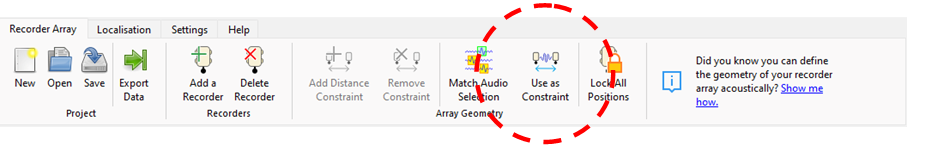
This converts the time difference between the recorders into physical distance constraints between the recorders.
Repeat these steps for the other calibration sounds you made. Once you have done this for a few recorders it should give you a reasonably accurate estimate of your array geometry.
 |  |
Localizing sounds:
Once your array geometry is well defined, localizing sounds is quite easy.
Draw a box around the sound you want to locate. Make sure the sound selection isn’t too long, only a few seconds or so max.

You might want to zoom in on the spectrogram in the x and y axis to find the sound. Press CTRL and use the scroll wheel of the mouse to zoom in/out around the frequency under the cursor. Selecting only the frequency band of your sound of interest improves the result of the calculations because it removes all the other sounds you are not interested in. Press the green play button to hear the filtered version of the selected sound to make sure it is the sound you are looking for.
Click the Find on Map button from the Localization tab of the main menu bar.

This will generate a cross-correlation map at each point across the area of interest. You can adjust the area of interest by dragging the edges of the grey bounding box.
The sound will be located where the lines of cross-correlation overlap, as shown by the green marker on the map below.

If you are happy with the result, you can give it a label or select a different icon. If you are happy with the result, click the Add to List button in the localization results table.
You can review past results by selecting them from the results table, at it will show the position and saved cross-correlation map.
Additional information:
A good result from clear signals will appear as obvious lines which overlap at a point. You can have confidence in the accuracy of results like these.
A noisy cross-correlation map is a sign of a bad match, either because the signals were poor or not located within the computed area. In this case you should try selecting a different part of the signal or find another clearer call to work with.

Exporting the results:
To use your results in an external program:
Click Export Data button from the main menu.

This will save the table of found sounds as a .csv file, which you can open in Excel.
For each located sound, it will save the following information:
Name, Latitude, Longitude, Altitude(relative), Date/Time, Filename, File Offset
While our software is still in development, here is a list existing acoustic localization software that you might like to investigate. *Note that these software packages do not perform the drift compensation described above and you will need to write some software to interpolate the samples.
PAMGUARD (Open source) - Designed for Dolphins and Whales. Has been around for a while. Good documentation, lots of features.
OpenSoundScape (Open source) - Library of python modules for analysing bioacoustic data. Contains routines for acoustic localization.
Ishmael (Free) - Open access bioacoustics analysis software, including localization facilities.
This is a living document prepared by Michael Maggs and will be updated over time as more information becomes available. If you have any questions or feedback, please reach out to me at: michaelm@frontierlabs.com.au +61 420757476 (Time zone UTC+10)


I would argue that the methodology is applied transparently and consistently. The reasoning is clear and well-founded. The website verifies and expands on the core findings presented. Contextual breadth is expanded through interactive service frameworks.
Really enjoyed this overview of acoustic localisation, especially the clear explanation of using TDoA across multiple recorders to recover a 3D source location. The sections on array geometry and ground-truthing make the practical steps feel much less mysterious, and the emphasis on processing choices should help anyone designing a solid project. Also appreciated the mention of CSV to JSON for handling outputs like CSV to JSON—being able to convert and validate formats quickly is a real productivity boost when you’re iterating on localisation results.
I really enjoyed this article, especially the part where it explains how acoustic localisation can pinpoint the direction of a sound using multiple sensors. That detail made the concept feel a lot more tangible, rather than just theoretical. I also appreciated the discussion about the challenges of noise interference and how signal processing helps improve accuracy it made me realize how complex real-world applications can be. Reading this reminded me a bit of the analytical thinking needed in my own studies, and sometimes I rely on resources like Assignment Help Websites to clarify tricky concepts in a clear way. I’m now curious about how this technology could be adapted for more everyday applications, like improving smart home systems or even…